Time Traveling with Data Science: Focusing on Change Point Detection in Time Series Analysis (Part 2)

In the first blog post of our „Time traveling with data science“ series, we presented several tasks related to the analysis of time series. In this post, we dive into the task called „change point detection“.  

Changes in time series or signals can take different forms. Roughly speaking, a change point is an abrupt change in a time series, meaning a change in the underlying trends, frequencies, or probability distributions.

Change point detection: Different types of change points 

Change point detection has a number of various applications. It is used, for example, in the fields of medicine, aerospace, finance, business, meteorology, and entertainment. Usually, change points are described in terms of changes between segments. To put it simple, a change point divides a time series into two segments where each segment has its own statistical characteristics (e.g., mean, variance, etc.). Thus, the change point is located where the underlying characteristics change abruptly. An overview of the most common change points and approaches for detecting them can be found in (Aminikhanghahi and Cook 2017; Truong et al. 2020). A theoretical description of change point detection, including the mathematical background, can be found in (Basseville and Nikiforov 1993). In the following, we will present some important examples of  change points. 

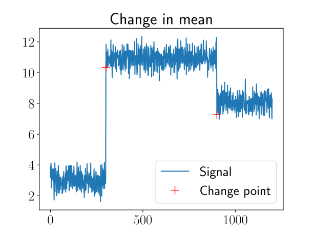
Change in mean is the most common example and probably also the easiest to identify (at least visually). Change in mean usually occurs when a time series can be divided into different constant segments having different mean values. One of the earliest algorithms for detecting such changes is the Cumsum algorithm (Page 1954), which was developed to detect change in mean. It was applied for quality control in manufacturing. 

 

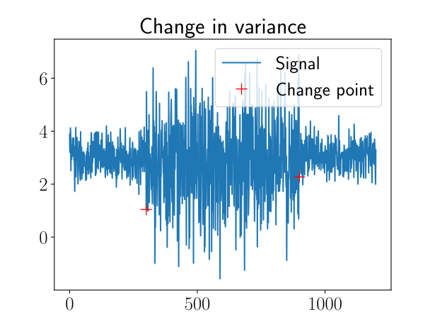
Change in variance is another famous example. Here, the mean value of the signal stays constant, but there are several segments with different variance values. This can be interpreted as a sudden noise in the signal. Both change in mean and change in variance can be detected by comparing statistical properties through the signal. 

 

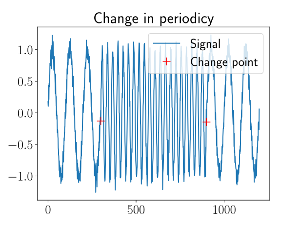
Change in periodicity (also called change in frequency) concerns time series with cyclic properties (e.g., a machine’s regime). Here, the change occurs when the frequency changes suddenly. Detection of this kind of change is usually done in the frequency domain, for example by using Fourier transform or wavelet transform.  

 

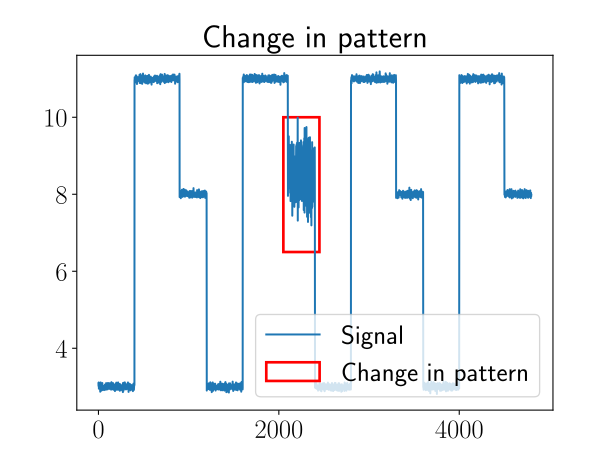
Change in pattern is more difficult to tackle than the previous ones. Such changes can occur, for example, in ECG signals. Ond one way to detect them is to use Wasserstein distances between empirical distributions (Shvetsov et al. 2020). At this point, we can see that change point detection is closely related to anomaly detection; the difference between the two tasks is sometimes fuzzy.

 

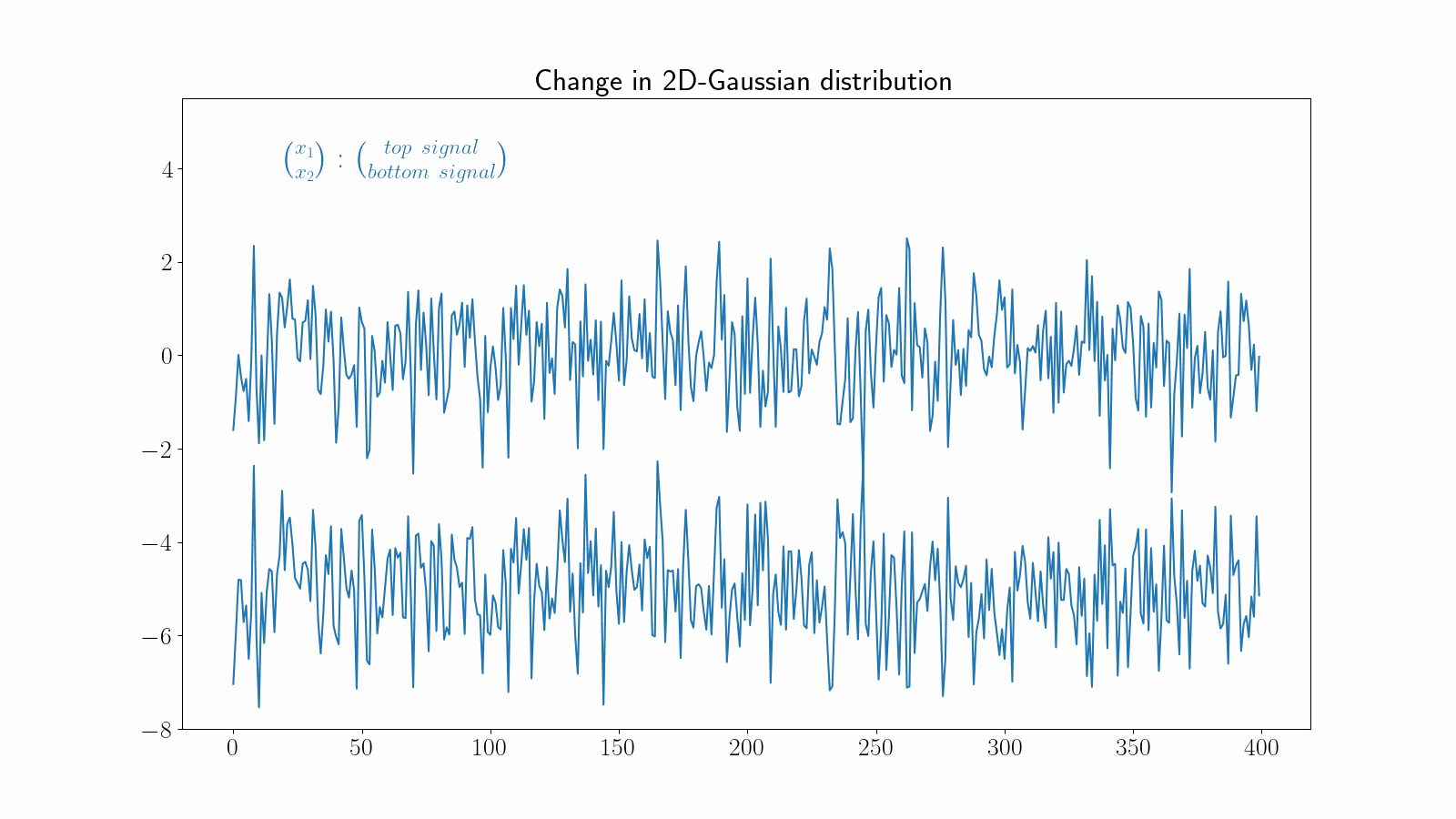
Changes in multidimensional time series can become very challenging to detect visually. The following example illustrates a change in the correlation between two dimensions of a time series. 

 

There are many other types of change points, depending on the underlying structure of the signal. Usually, the more complex the signal, the more difficult it is to detect the change point.  

Detecting change points 

There are countless ways and methods for detecting change points that have been developed during the last decades. An overview of the most common approaches can be found in (Aminikhanghahi and Cook 2017). Several packages for detecting change points have been implemented in R and Python. Usually, most packages provide a lot of hyperparameters that can be adjusted to optimize change point detection or even optimize runtime. However, many packages are not standardized: Some only calculate the costs but not the actual change points, while other packages are not maintained regularly.

Well-known, established, and regularly maintained examples of packages are: 

• In R, the following packages are dedicated to change point detection: changepoint, kcpRS, or bcp.
• In Python, the ruptures packages are completely dedicated to change point detection. Other packages such as prophet, luminaire, and scikit-multiflow include – among other features – change point or drift detection. 

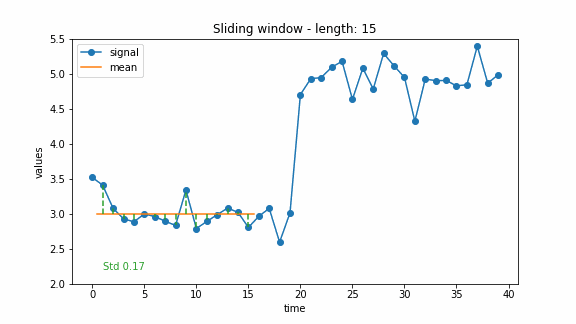
A common way to conduct change point detection is a sliding window through the signal. The main idea is to walk through the signal with a window of fixed size. For each step, a function computes a chance of having a change point in the current window. This function is usually called the cost function. Thus, for each point in the signal, we obtain a cost value indicating whether there is a change at that point or not. Usually, the costs are “low” as long as there is no change in the window and “high” if there is a change in the window. For example, if the costs exceed a pre-defined threshold, the point is marked as a change point, or the points with the highest costs can be marked as change points. 

To detect changes in mean, a simple approach is to use the standard deviation as a cost function. As long as the signal is constant (with some noise), the standard deviation is low. If there is a jump in the signal, the standard deviation will rise. The animation below shows an example of calculating the costs of a change in mean using the standard deviation.  

 

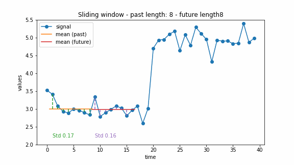
The window-based approach can have different extensions. For example, there can be two windows, a past one and a future one. Then the change point can be detected by comparing the costs of these two windows. This idea was also used for the the generalized log-likelihood ratio test (Basseville and Nikiforov 1993). The example below illustrates this approach. 

 

How to choose an appropriate method for change point detection

The theory of change point detection is well established in the literature; several methods have been implemented in standard packages. The question of how to choose the right one is crucial and depends on many factors. As there are many approaches and methods, we present three important factors to make a reasonable decision.

First, you need to know your signal and which type of change you have. Obviously, not every software package can deal with every kind of change. For example, the bcp package in R was developed for sequencing DNA series using a Bayesian approach. But this package cannot be applied to detect changes in mean for normally distributed random variables because it will deliver too many false positives.

Second, the runtime plays an important role. Depending on the application, sensors may deliver hundreds of points in one second. The window-based methods presented above have a runtime of O(T), where T denotes the length of the signal. That is the reason why most of these types of algorithms can be used in online applications. As more and more data is produced in the context of IoT, much research has been done in the field of online change point detection in the last few years; see, for example, (Namoano et al. 2019). However, such window-based algorithms are usually approximations and therefore often deliver too many change points, which leads to the next factor.

Third, some applications require accurate results. There are other approaches that need a longer runtime but deliver more precise change points. Famous methods are, for example, the binary segmentation or bottom-up approaches, which take O(T log(T)) time, but they are still approximations. Exact methods take at least O(T²), some even O(T³) time. At this point, it should be mentioned that some methods are very advantageous if one knows how many change points are present in the signal because they stop with an optimized solution. But for many applications with continuous sensor data, this is not realistic.

In our next series, we will deal with other exciting topics regarding time series analysis. There are many other tasks (for example, classification, clustering, blind source separation) that are also highly relevant in applications. We will also present ideas on how to tackle these tasks. Stay tuned!

References

[1] Aminikhanghahi, Samaneh; Cook, Diane J. (2017): A Survey of Methods for Time Series Change Point Detection. In Knowledge and information systems 51 (2), pp. 339–367. DOI: 10.1007/s10115-016-0987-z.
[2] Basseville, M.; Nikiforov, Igorʹ V. (1993): Detection of abrupt changes. Theory and application /  Michèle Basseville, Igor V. Nikiforov. Englewood Cliffs, N.J.: Prentice Hall; London :  Prentice-Hall International (Prentice Hall information and system sciences series). Available online at http://people.irisa.fr/Michele.Basseville/kniga/kniga.pdf.
[3] Namoano, Bernadin; Starr, Andrew; Emmanouilidis, Christos; Cristobal, Ruiz Carcel (2019 – 2019): Online change detection techniques in time series: An overview. In : 2019 IEEE International Conference on Prognostics and Health Management (ICPHM). 2019 IEEE International Conference on Prognostics and Health Management (ICPHM). San Francisco, CA, USA, 17.06.2019 – 20.06.2019: IEEE, pp. 1–10, checked on 4/8/2021.
[4] Page, E. S. (1954): Contiuous Inspection Schemes. In Biometrika 41 (1-2), pp. 100–115. DOI: 10.1093/biomet/41.1-2.100.
[5] Shvetsov, Nikolay; Buzun, Nazar; Dylov, Dmitry V. (2020): Unsupervised non-parametric change point detection in quasi-periodic signals, checked on 11/25/2020.
[6] Truong, Charles; Oudre, Laurent; Vayatis, Nicolas (2020): Selective review of offline change point detection methods. In Signal Processing 167, p. 107299. DOI: 10.1016/j.sigpro.2019.107299.