
In our last Fraunhofer IESE blog post, we introduced a holistic process planning and scheduling design called RL design, which addresses individualized production with small lot sizes. However, this design cannot deal with scheduling problems in the case of large job quantities. In this post, we introduce the second RL design: process planning with subsequent scheduling. This design aims to address the case where jobs arrive continuously at random times, with all of them sharing several common product types.
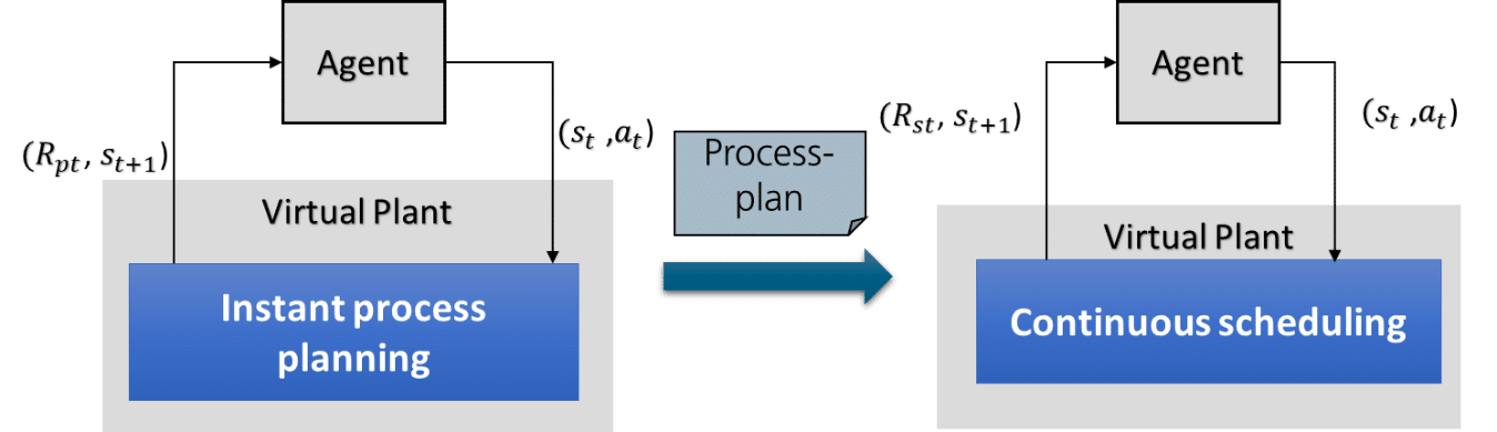
This design separates the process planning module and the scheduling modules into two separate DQN architectures. The DQN for process planning is started first. It has the same construction as the first RL design except that all services have a duration of a single time step and the agents only have to learn to synthesize process plans instead of deriving schedules. This reduces the computation time for process planning dramatically. The process plans are stored in one place and are later accessed by the scheduling module. The continuous scheduling module is responsible for deriving near-optimal schedules based on the process plans.
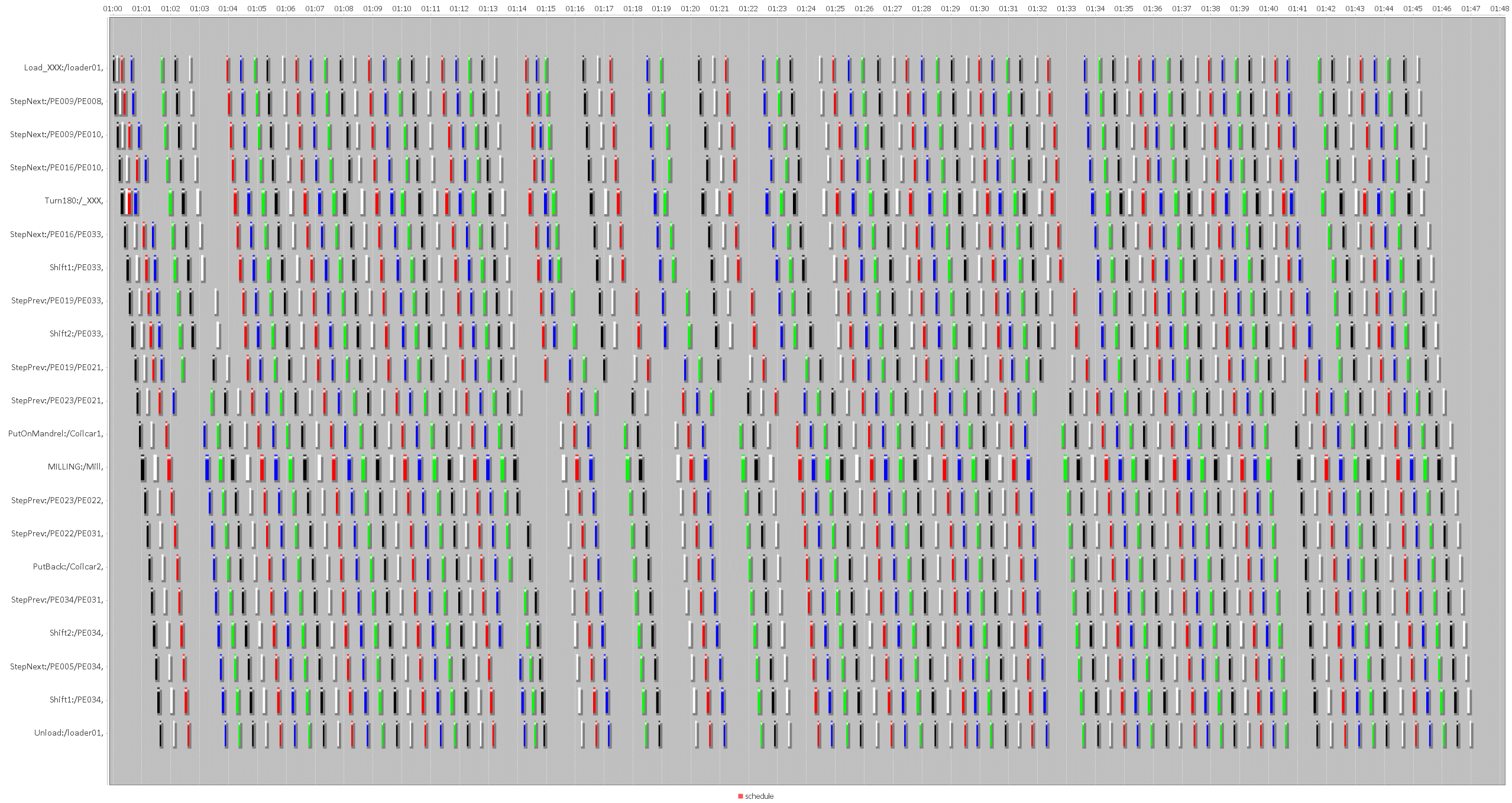
Process planning and scheduling for large job quantities
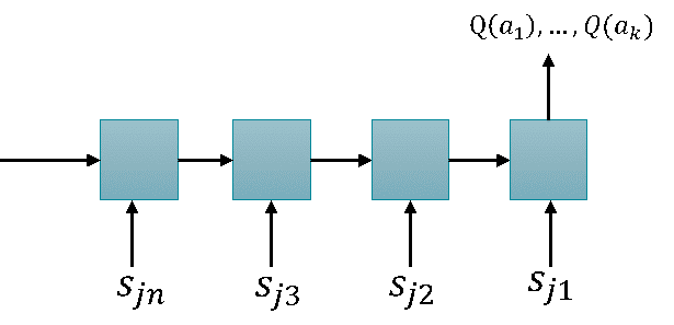
The DQN for continuous scheduling has a different RL design, especially for state space modeling and reward generation. The action space of this design can still be formulated as A= {a_1, a_2, a_3, …, a_k}Ua_{idle}. The state space contains only the job states S={s_{j1}, s_{j2},…,s_{jn}}. Each job state contains the following information: (1) current services based on the process plan. The current services of all jobs form a set a_{cur} = {a_{cur(j1)}, a_{cur(j2)}, …, a_{cur(jn)}}; (2) the service providers of the current services; and (3) the current status of the service providers. In this state modeling, the resource state is represented implicitly inside a job state. This design uses a Long-Short-Term-Memory (LSTM) network as the approximation function, where the series of job states are fed into the input series of the LSTM. The output equals the quality values of the actions.
Rewarding system
The reward modeling of this design is application-specific. It can be summarized as follows: (1) The virtual plant checks whether the selected service belongs to the set of current services A_{cur}. If this is not the case, a negative reward is returned to the agent. (2) If the selected service belongs to A_{cur}, the virtual plant checks the executability of the service using the logic shown in Figure 4. If the service is not executable in the current state, a negative reward is returned to the agent. (4) Otherwise, the service is started at the current time step. Now the logic of the scheduling module is started to manage the running services and a scheduling reward is generated based on the mean machine utilization. (5) Finally, it checks whether new jobs arrive at the current time step. The released jobs are added to the internal queue of the virtual plant and are ready for scheduling.
Validation and result analysis
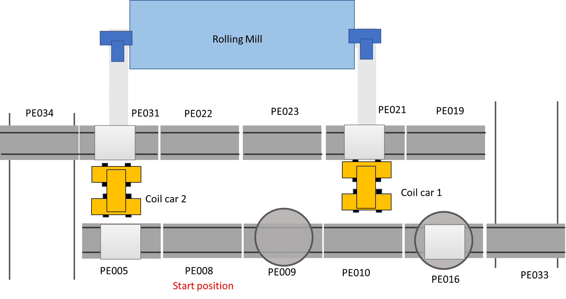
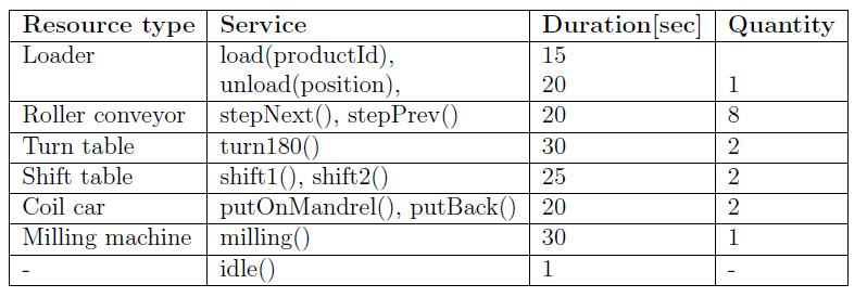
We performed a case study using a virtual aluminum cold rolling mill, which is shown in Figure 3. It consists of a cold rolling mill and a pallet transport system. The pallet transport system consists of multiple roller conveyors, turn tables, and shift tables to move an aluminum coil to a specific position. All resource types and their services are shown in Table 1.
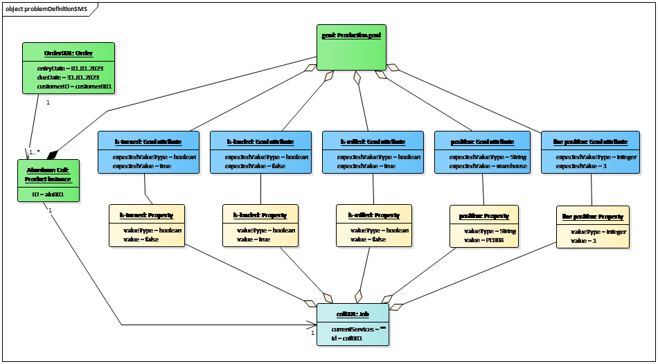
The aluminum coils should be transported to the cold rolling mill and transported back to the warehouse after the milling process. Figure 4 shows the modeling of the production goal of an aluminum coil. This production goal defines that the coil should be turned by a turn table (“is-tuned=true”) and processed by a rolling mill (“is-rolled = true”). The job properties that are represented as the yellow boxes show the current job state of the aluminum coil. The agent tries to find a sequence of services that can change the jobs states to the values defined in the production goal.
Results
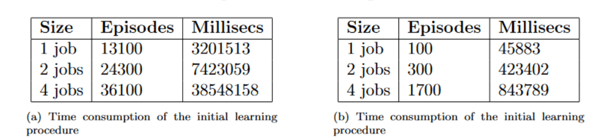
The evaluation focused on the scalability of our approach with different numbers of jobs. Hence, we measured the time the agents need for the initial and repeated learning process. The experiment was performed on a computer with an Intel i5 core with 4G RAM. The neural networks had a CPU backend. Figure 5 shows the time consumption for the 1st RL design. For the initial learning process, the agent needed about 40 min. to learn the process plans for a single job, about 2 hours for 2 jobs, and more than 10 hours for 4 jobs. For the repeated learning process, where the agent should learn new schedules for different production goals, the agent only needed about 10 min to derive schedules for 4 jobs. From the statistics, we can see that this design is adequate for individualized production with small lot sizes.
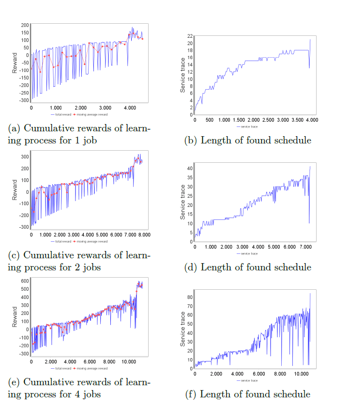
In the evaluation of the second RL design, the agents took about 16 hours for the initial learning round. During the learning process, the production performance KPIs improved continuously. The average job flow time decreased from about 1250 s to about 550 s; mean machine utilization increased from about 0.015 to around 0.5.
One significant discovery of this experiment for the second RL design was that a trained agent can handle a range of situations without re-training. We summarize the factors as follows:
- No re-training required:
- Job release period
- Job release timepoint
- Job release quantity
- Service duration
- Re-training necessary:
- Changing of production goals, where new product types are inserted.
- Changing of available resources and services.
Conclusion
We have presented two RL designs and performed a validation for both RL designs. The validation results show that the first RL design is suitable for individualized production with small lot sizes where process plans are adapted frequently due to the introduction of new product types. The second RL design is suitable for problems with large job quantities where jobs arrive continuously at random times.
Bibliography
[1] D. Silver, T. Hubert, J. Schrittwieser, I. Antonoglou, M. Lai, A. Guez, M. Lanctot, L. Sifre, D. Kumaran und T. &. o. Graepel, „A general reinforcement learning algorithm that masters chess, shogi, and Go through self-play,“ Science, 2018.
[2] „ChatGPT: Optimizing Language Models for Dialogue,“ OpenAI, [Online]. Available: https://openai.com/blog/chatgpt/
[3] V. Mnih, K. Kavukcuoglu, D. Silver, A. Graves, I. Antonoglou und D. &. R. M. Wierstra, „Playing atari with deep reinforcement learning,“ arXiv preprint arXiv:1312.5602, 2013.
[4] B. M. a. Y. G. Kayhan, „Reinforcement learning applications to machine scheduling problems: a comprehensive literature review,“ Journal of Intelligent Manufacturing, pp. 1–25, 2021.
[5] T. a. S. F. a. O. A. P. Kuhn, „Service-Based Architectures in Production Systems: Challenges, Solutions amp; Experiences,“ in 2020 ITU Kaleidoscope: Industry-Driven Digital Transformation (ITU K), 2020.

